Mini-vLLM and CARL
An LLM serving engine written from scratch around TinyLlama-1.1B, so that every idea inside vLLM is visible and testable. Then an online controller that reconfigures it while it runs, and a careful answer to whether that controller helps.
- Role
- Sole engineer and author
- Timeline
- Jan 2026 to present
- Status
- Manuscript under review, MLSys 2027
- Stack
- Python, PyTorch, Triton, FastAPI, Prometheus, Grafana, Docker
Serving is a scheduling problem
Generating text with an LLM happens in two phases. Prefill pushes the whole prompt through the model at once and is compute-bound. Decode then produces one token per step per request and is limited by memory bandwidth, because every step rereads the weights and the request's key/value cache.
A server has to decide, every step, which requests run, how much prompt to prefill, and where each request's KV cache lives in a fixed amount of GPU memory. Get it wrong and the GPU idles between requests, or one long prompt freezes everyone else's tokens, or memory fragments until nothing new fits. vLLM's answers are continuous batching and a paged KV cache. I wanted to understand those answers well enough to rebuild them, test them against Hugging Face, and then ask a research question on top.
Explore the engine
This is a small simulation of the same mechanisms, running in your browser. Switch the policy to see what each technique fixes. Hover a request to see its KV blocks light up in the cache. The numbers it shows are simulated; the measured results are in the next sections.
Scheduling policy
Workload
What to watch
Finished requests leave and new ones join at every step. Without chunking, any step with prefill work runs only prefill, so a long prompt stalls every decode for that step. Look for the GPU step flipping between prefill and decode.
What I built
Everything below the FastAPI layer is hand-written: the model, the attention, the cache and the scheduler. Each layer has a parity test against transformers at atol=1e-4, so a faster path is only accepted if it produces the same tokens. The suite has about 830 tests.
- Model
- Llama architecture from scratch: RoPE, grouped-query attention, SwiGLU, RMSNorm in fp32. A fused Triton RoPE kernel with numerical parity tests against the PyTorch version.
- Paged KV cache
- 16-token blocks in split K and V pools, stored layer-major with block size before KV heads, so attention reads views instead of strided copies. Each layer tracks its own cache length, which fixed an off-by-one in cached generation.
- Scheduler
- Continuous batching with admission control under block pressure, a priority and deadline-aware SLA scheduler, chunked prefill with a per-step token budget, and a radix-tree prefix cache.
- Speculative decoding
- Self-speculation by early exit, with KV rewind and byte-identical output to greedy decoding. Off by default, for reasons shown below.
- Experimental paths
- CUDA Graph decode, multi-LoRA adapter routing, W8A8 quantisation, FlashAttention, disaggregated prefill and decode, each with its own benchmark script. I do not quote numbers for them here because their raw logs are not committed.
- Observability
- Prometheus metrics and a pre-provisioned Grafana dashboard: TTFT and TPOT percentiles, queue depth, KV utilisation, batch-size heatmap, CUDA Graph hit rate, and the profiler's bottleneck over time. A WebSocket visualiser streams every scheduler event.
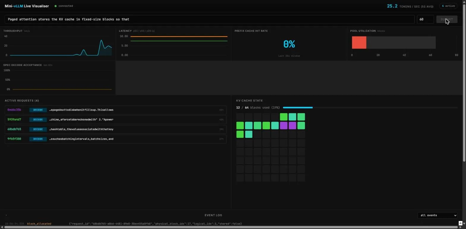
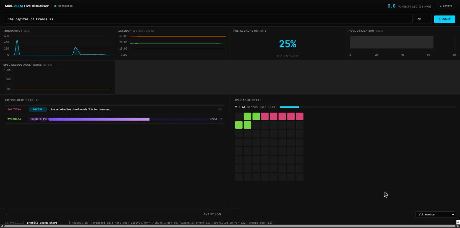
Measured results
Three measurements with committed raw logs. They are small and specific on purpose: one laptop GPU or one T4, one 1.1B model, fp32 where parity matters.
Aggregate throughput
- Sequential generate()24.4 tok/s
- Continuous batching, 64 KV blocks44.6 tok/s
- Continuous batching, 6 KV blocks33.3 tok/s
Prefill latency, ms
Speedup over plain decoding
The speculative decoding result is a negative one, and I kept it. The machinery is correct (it matches greedy output byte for byte), so the path forward is a trained draft mechanism such as a LayerSkip fine-tune or an EAGLE-style head, not more tuning. A separate comparison script runs both engines on identical workloads; Mini-vLLM is roughly an order of magnitude slower per token than vLLM, and each part of that gap maps to a technique I left out for readability.
CARL: does online tuning help?
Serving engines expose knobs such as the maximum batch size and the prefill chunk size. They are usually tuned offline and frozen. CARL is the alternative: a regime classifier plus a LinUCB contextual bandit per regime, choosing from a table of configurations while the engine runs.
The question is easy to ask unfairly. A static baseline can be tuned for the wrong objective, a reward can depend on latencies not yet measured, and “convergence” can be read off a controller that never explored. So the final study varies only the two knobs verified to be live, picks static baselines by exhaustive search of all 28 configurations on a held-out seed, withholds rewards built from unmeasured latencies, and compares paired runs over ten seeds.
Saturated burst, Tesla T4, TinyLlama-1.1B, fp16, 200 requests per run.
Each row is the first system minus the second, paired by seed, with a 95% interval. Learning beats a fixed rule, but the controller stays below static configurations picked offline for the same objective, and a wider action space makes things worse. Source: the frozen section of the project's claim ledger.
Relative throughput range, %
- Saturated burst53.15 %
- Sub-critical, S10.39 %
- Sub-critical, S20.75 %
- Sub-critical, O0.32 %
Mean time per component, µs
- Arm selection (LinUCB)49.4
- Context and classification14.5
- Reward computation11.4
- Apply configuration3.5
- Logging1.0
The finding. At the saturated operating point, learning is worth +3.76 tok/s over a fixed rule with the same classifier and arm table (95% CI +3.29 to +4.23), but the controller stays below static configurations chosen offline for the same objective. At a sub-critical Poisson load it trails both on end-of-run utility. No run in any treatment met the pre-stated convergence diagnostic. These findings are about this system, one model and one GPU, not about online adaptation in general.
What I took back
An earlier draft of this work claimed that CARL reached 108% of a tuned static configuration, converged deterministically at cycle 9, and had an effect size of d = 23. I wrote a claim ledger that checked every sentence against the repository's own artifacts. Those claims, and several others, did not survive.
- The reward was constant
- On the GPU, reward v1 took exactly two values ever: 0.8 for three cycles, then 0.3 forever. All four terms were pinned by their clips. A bandit cannot learn from a constant, which also explained why three “independent” seeds were byte-identical.
- The bandit never explored
- At α = 0.5, untried arms scored zero against strictly positive rewards, so LinUCB played arm 0 every time. Adding an intercept feature and centring the reward fixed it; removing both reproduced the lock-in exactly, as a test.
- The baseline was circular
- In the old simulator the oracle, the bandit's first arm and most static candidates were the same configuration. It was replaced by a substrate that imports nothing from the controller, which a test asserts.
- The workload flattered tails
- Dumping 25 requests at once behind a concurrency cap turned queueing delay into apparent tail-latency wins. Poisson arrivals at a derived load replaced it.
This was not the paper I set out to write. It is a better one: the methods that caught these problems (a null ablation that freezes learning, a circularity check, and an arm-set coverage check) are cheap and would have caught them on day one.
Decisions and trade-offs
- fp32 for parity
- Running in fp32 lets every layer match Hugging Face at 1e-4. It roughly doubles memory traffic in a bandwidth-bound decode, which is part of the gap to vLLM. Correctness first, then speed behind a test.
- Python step loop
- Readable and easy to instrument, but host overhead grows with batch size. vLLM's C++ scheduler and CUDA Graph replay are the production answers; the profiler shows where this engine pays for the choice.
- Synchronous event bus
- The scheduler emits events synchronously from worker threads, and each WebSocket subscriber owns an asyncio queue fed through call_soon_threadsafe. The bus never needs to know about asyncio.
- Speculation off by default
- At measured acceptance rates, enabling it slows every request. The interface stays so a trained draft head can be dropped in.
- Reproducible GPU runs
- Colab runs with incremental checkpoints, verified resume after interruption, and SHA-256 hashes for source and artifacts, so a result can be traced to the exact code that produced it.
Lessons
Correctness tests against a reference implementation are what made the engine trustworthy enough to experiment on. Without them, every speed-up would have been a guess.
On the research side, the most useful thing I built was not the controller but the ledger: a table where each claim has evidence and a status, and where a contradicted claim is retracted rather than softened. The final result is smaller than the first draft and I trust all of it.